Viral Math

The goal of epidemiologists is first to understand the causes of a disease, then to predict its course, and finally to develop ways of controlling or eliminating it. Within the larger scientific study, the subfield of mathematical epidemiology uses mathematics to model how diseases will spread, their rate of growth, and the effectiveness of potential treatments. Models let us extrapolate out from an observed data set—without any of the ethical quandaries caused by conducting medical experiments on human subjects—to study patterns and make predictions about how quickly a particular disease may infect a given population, which can then influence critical decisions about medical care.

Dating back to the 18th century, mathematical epidemiology draws on statistics, probabilistic math, calculus, and differential equations, among other domains. The field’s power to model epidemics and forecast the effects of potential treatment courses has been greatly enhanced by modern computers. Digital technologies have increased the speed and computing power applied to standard mathematical models, while also allowing for vastly more complex simulations of a pandemic.

At present, the fast-spreading coronavirus, which has led to a state of emergency across the United States and much of Asia and Europe, has also spurred considerable effort among mathematical epidemiologists. The research group at the London School of Hygiene and Tropical Medicine has been at the forefront of the coronavirus modeling, and its contributions have been circulated widely, but many other groups and individuals all over the world have also contributed. The basic models being used are the so-called compartmental models that date back to 1927, but there have been significant advances in the methods of estimating model parameters from observed data. Those advances are especially applicable when the data are incomplete and unreliable as they are in this case with numbers coming in from countries all over the world, not all of them fully transparent in their reporting about the disease.

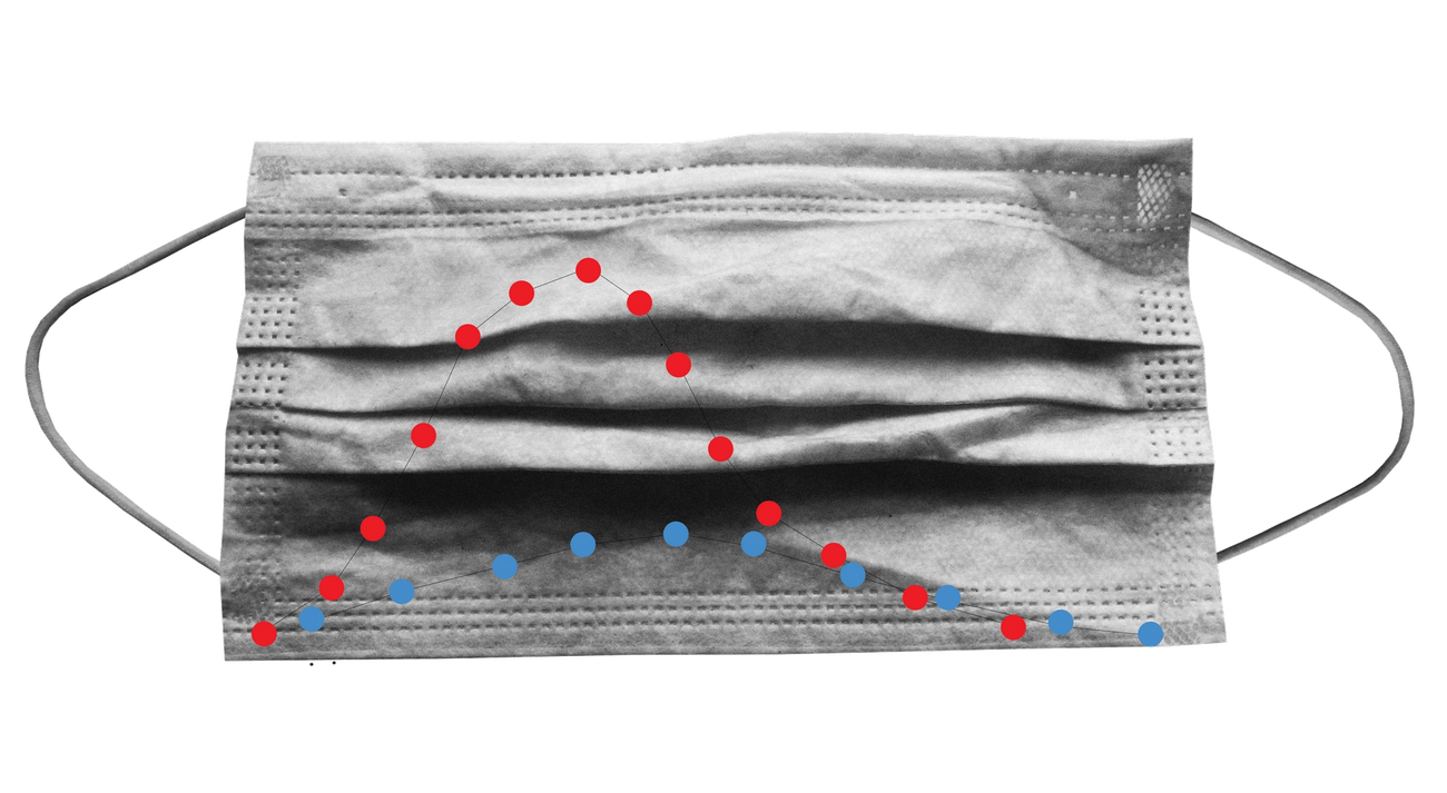
Another example of newly popularized mathematical epidemiology is the U.S. Centers for Disease Control and Prevention’s “flattening the curve” graph, which has achieved its own viral status as a meme. The original CDC graph dates back to 2007 but has gone through several updates and iterations on the way to its current popularity. The image portrays two differential outcomes for the progress of coronavirus in the United States. In one scenario, the disease continues its spread unimpeded, leading to a dramatic spike bound to overwhelm the health care system. In the alternate, “flattened” scenario the rate of transmission is slowed through mitigating measures, preventing hospitals from being inundated, preserving the supply of critical medical inventory and allowing doctors to give sick patients proper care.

Important to remember that #Covid-19 epidemic control measures may only delay cases, not prevent. However, this helps limit surge and gives hospitals time to prepare and manage. It’s the difference between finding an ICU bed & ventilator or being treated in the parking lot tent. pic.twitter.com/VOyfBcLMus

— Drew A. Harris, DPM, MPH (@drewaharris), February 28, 2020

The study of infectious disease data began with the work of John Graunt (1620–1674) in his 1662 book Natural and Political Observations made upon the Bills of Mortality. The Bills of Mortality were weekly records of numbers and causes of death in London parishes. The records, beginning in 1592 and kept continuously from 1603 on, provided the data that Graunt used. He analyzed the various causes of death and gave a method of estimating the comparative risks of dying from various diseases, giving the first approach to a theory of competing risks.

What is usually described as the first model in mathematical epidemiology is the work of Daniel Bernoulli (1700–1782) on inoculation against smallpox, which was epidemic in the 18th century. Variolation, essentially inoculation with a mild strain, was introduced as a way to produce lifelong immunity against smallpox, but with a small risk of infection and death. There was heated debate about variolation, and Bernoulli was led to study the question of whether variolation was beneficial. His approach was to calculate the increase in life expectancy if smallpox could be eliminated as a cause of death. His approach to the question of competing risks led to publication of a brief outline in 1760 followed in 1766 by a more complete exposition.

Another valuable contribution to the understanding of infectious diseases was the knowledge obtained by study of the temporal and spatial pattern of cholera cases in the 1855 epidemic in London by John Snow, who was able to pinpoint the Broad Street water pump as the source of the infection. In 1873, William Budd gained a similar understanding of the spread of typhoid. In 1840, William Farr studied statistical returns with the goal of discovering the laws that underlie the rise and fall of epidemics.

A striking example of pioneering mathematical epidemiology is the work of Sir R.A. Ross, who received the second Nobel Prize in medicine in 1902 for showing that malaria was transmitted from human to human through mosquitoes. Although this work received immediate acceptance in the medical community, his conclusion that malaria could be controlled by controlling mosquitoes was dismissed on the argument that it would be impossible to rid a region of mosquitoes completely. After Ross formulated a mathematical model in 1911 predicting that malaria outbreaks could be avoided if the mosquito population could be reduced below a critical threshold level, field trials supported this conclusion and led to some brilliant successes in malaria control. Unfortunately, mosquitoes have resisted efforts to control them and that, combined with people becoming resistant to pharmaceuticals, has made malaria an ongoing problem into the 21st century.

Today, basic mathematical theory for epidemics relies on what are known as compartmental models that are applicable if the population being studied is homogeneous, that is, if the behavior of all members is the same. In fact, this never actually exists since all populations are heterogenous, with variables like contact and recovery rates depending on age. But the models can be adapted to account for this by dividing the population into subgroups with different behaviors, including assumptions on the rate of mixing between different groups. It is even possible to study an agent-based model, which essentially tracks each individual, and advance made feasible by the invention of high-speed computers.

W.O Kermack and A.G. McKendrick, a Scottish biochemist and epidemiologist, respectively, were key figures in the evolution of the math behind viral growth. Between 1927 and 1933, their work on compartmental models for general classes of diseases, made it possible to obtain important information using only relatively simple mathematics. By dividing the population under study into compartments, labelled S, I, and R, they could make assumptions about the nature and time rate of transfer from one compartment to another: S denotes the number of individuals susceptible to the disease, who are not (yet) infected; I denotes the number of infected individuals, who are infectious and can spread the disease by contact with susceptibles; and R denotes the number of individuals who have been infected and then removed from the possibility of being infected again or of spreading infection.

The compartmental approach works for modeling both epidemics—the sudden outbreak of a disease that infects part, but not all, of a population, before disappearing—and endemic diseases, which remain present in a population.

The essential difference between an endemic disease and an epidemic is that in an endemic disease there is a mechanism for a flow of new susceptibles—that is people at risk of catching the disease—into the population. This may result in a level of infection that remains in the population. In an epidemic, there is no flow of new susceptibles into the population and the number of infectives—people infected with the disease—eventually decreases to zero.

In some diseases, the disease confers no immunity against reinfection and infectives return to the susceptible class on recovery. The acronym SIR is used to describe a disease which confers immunity against reinfection, to indicate that the passage of individuals is from the susceptible class S to the infective class I to the removed class R. The acronym SIS describes a disease with no immunity against reinfection, to indicate that the passage of individuals is from the susceptible class to the infective class and then back to the susceptible class.

In addition to the basic distinction between SIR and SIS models, there are SIRS models, indicating temporary immunity, SEIR models, with an exposed period between being infected and becoming infective, and SITR models, in which a fraction of the infectives are selected for treatment.

The critical threshold introduced by Ross for malaria is called the basic reproduction number, denoted by R₀ and defined to be the number of secondary infections caused by introducing a single infective into a wholly susceptible population. This is a central quantity in mathematical epidemiology depending on the rates of transition between compartments in any model; there are mathematical techniques for calculating the basic reproduction number in any model.

In an epidemic model, if R₀ < 1, the infection will die out, while if R₀ > 1,there will be an epidemic; that is, the number of infectives will grow initially before eventually dying out.

For an SIR epidemic model, the size of each compartment approaches a limit as time becomes large; there is a limiting number of susceptibles S* > 0, and the number of infectives goes to zero.

Early in an epidemic, almost all contacts by an infective are with people susceptible to infection and produce new infections. As a result, the number of infectives grows exponentially. Later in the epidemic some contacts by an infective are with someone who has already been infected and these do not produce new infections, so the curve levels off. The non-randomness of contacts affects the rate but isn’t the main reason for the tapering off of new disease cases.

For an endemic disease SIR model the process of analysis is quite different. Usually (but not always), both S and I approach limits S* and I* respectively. If R₀ > 1, the limiting infective population size is positive, and the disease remains in the population, but if R₀ < 1 the limiting infective population size is zero, and the number of infectives dies out.

The point is that if one knows the basic reproduction number, then one knows the course of the disease (although this is not quite true if the mixing in the population is not homogeneous).

In the Chinese city of Wuhan where the coronavirus originated, the R₀ had climbed to 3.86 in January. That number had reportedly decreased by more than 90% to 0.32 in early March following the far-reaching and radical interventions of the Chinese government, which have included locking down and surveilling tens of millions of people to control the spread of the disease.

In 2002 a new infectious disease appeared, first in China, that spread to other parts of the world, including Singapore, Taiwan, and the Greater Toronto Area of Canada. Initially, it was misdiagnosed as influenza but it was soon recognized as a new disease originating in chickens, and given the name SARS (severe acute respiratory syndrome).

There were immediate fears that SARS could be a major threat to public health. For a new disease, no medical treatments are available. The only control measures available are isolation of diagnosed infectives and quarantine of suspected exposed individuals, who may be identified by contact tracing of infectives. It turned out that such measures were sufficient to control the epidemic, which ultimately caused only about 8,000 deaths worldwide.

SARS actually turned out to be a “good” epidemic because it alerted the public health community to several new aspects of communicable disease, including:

• the possibility of rapid spread over long distances through air travel, which led to the development of metapopulation (populations of populations linked by travel between them) models,
• the recognition of heterogeneity of contacts and “superspreading” events such as the Amoy Gardens residential complex in Hong Kong where a failure of the drainage system led to 329 infections and 42 disease deaths. This led to the development of contact network models, and
• the importance of nosocomial (in-hospital) infections.

These factors led to new approaches to epidemic management that were applied to the concern about a possible H5N1 influenza pandemic in 2005 and an H1N1 influenza pandemic that actually did develop in 2009—killing approximately 60,000 persons in the United States alone.

It is now generally thought that superspreading is very common in epidemics, with a rough rule of thumb being that 20% of a population causes 80% of disease cases.

It is easy to incorporate vaccination into disease outbreak models—an especially important step if vaccination may have harmful side effects. This has been important in smallpox control and has also led to serious misinformation in vaccines for such diseases as measles. If there is a perfect vaccine that immunizes all treated individuals, then even immunization of a fraction of the population decreases the basic reproduction number to less than one. When vaccinations are introduced into an epidemic model, the result is that there is no epidemic, and for an endemic disease model the infection dies out. In either case, it is said that herd immunity has been achieved.

The basic reproduction number for smallpox is approximately 5. Vaccination of 80% of the population would provide herd immunity; this has been achieved worldwide. The basic reproduction number for measles is about 15, meaning that it would be necessary to vaccinate more than 93% of the population to achieve herd immunity, a goal that is probably impossible.

In practice, vaccines are never perfectly effective, and a proper model would require a more complicated model with separate compartments for vaccinated and unvaccinated individuals. There is still a critical immunization fraction for herd immunity, but the above herd immunity estimate is a reasonable first approximation.

The coronavirus is a class of virus related to the SARS virus as well as the Middle East respiratory syndrome (MERS), which appeared in 2012. So far, the virus has been isolated and analyzed, and efforts to develop a vaccine have started. However, efforts to develop a vaccine, a process that often takes more than a year, may be useful for a later outbreak but may not help with the current outbreak.

The strain of the coronavirus designated COVID-19 that first appeared in the Chinese city of Wuhan at some point late last year has grown rapidly and progressed from epidemic to pandemic—the latter being an epidemic that has spread to multiple regions across the world. On Jan. 31 there were 9,800 cases and 213 disease deaths reported in China, and 103 cases outside China, while on Feb. 1 there were 13,900 cases and 304 disease deaths reported in China and 158 cases outside China. By March 13 the number of reported cases in China had increased to 80,817 and the number of disease deaths in China had increased to 3,177, though accurate numbers have been suppressed by the Chinese government and are difficult to determine at the moment.

Outside of China, there are large numbers of disease cases in several countries. There are currently more than 17,000 cases in Italy and more than 11,000 reported cases in Iran—a number that is likely to be far higher, based on nongovernmental reporting.

The spread of coronavirus has been tracked mathematically by a model similar to the one developed for SARS. The basic model is an SEIR model, but it is not clear whether there may be some infectivity during the exposed stage or whether there is an asymptomatic group (individuals with infectivity but no symptoms).

One of the main management approaches suggested is social distancing, which refers to the reduction of contacts between people through behavioral changes. The West African Ebola outbreak of 2014, which had far fewer disease cases than were initially predicted by epidemic models, provides an example of the approach working in practice. A successful public messaging campaign created the widespread perception that the disease was a serious danger, which caused people to limit their interpersonal contacts. This was really the inception of the practice of social distancing.

Because it is impossible to estimate the extent that people will actually alter their contacts, it is not possible to estimate the effect on the final size of the epidemic. Thus ranges from 30% to 80% of epidemic size have been predicted by public health professionals, but these predictions are probably more guesswork than model predictions. If the decrease in contact rates as the epidemic proceeds can be measured, it would be possible to give a more accurate estimate. Because the data for COVID-19 is incomplete and unreliable, there has been a range of estimates of the reproduction number ranging from 2.2 to 3.11. When the data become more reliable, sharper estimates will be available.

In fact, modern technology may be making such measurements available to governments that have the means and political license to use them. In China, the combination of martial-law-like emergency measures and advanced tracking technologies like facial recognition programs allow the government to monitor and punish unsanctioned social interactions between people under quarantine. In Israel, meanwhile, the government recently authorized the Shin Bet security service to monitor the cellphone usage of citizens in order to detect interactions with people diagnosed with the virus. From a purely academic perspective, the vast troves of up-to-the-minute data available through modern technological surveillance approaches could dramatically improve the predictive accuracy of the math used to model epidemics. Whether such a tradeoff would be worth it, is a different sort of question far outside the domain of mathematics and epidemiology.